1. Introduction
Currently used research and commercial robots are able to navigate safely through their environment, avoiding static and dynamic obstacles. However, a key aspect of mobile robots is the ability to navigate and manoeuvre safely around humans [
1]. Mere obstacle avoidance is not sufficient in those situations because humans have special needs and requirements to feel safe and comfortable around robots. Human-Robot Spatial Interaction (HRSI) is the study of joint movement of robots and humans through space and the social signals governing these interactions. It is concerned with the investigation of models of the ways humans and robots manage their motions in vicinity to each other. These encounters might, for example, be so-called
pass-by situations where human and robot aim to pass through a corridor trying to circumvent each other given spatial constraints. In order to resolve these kinds of situations and pass through the corridor, the human and the robot need to be aware of their mutual goals and have to have a way of negotiating who goes first or who goes to which side. Our work therefore aims to equip a mobile robot with understanding of such HRSI situations and enable it to act accordingly.
In early works on mobile robotics, humans have merely been regarded as static obstacles [
2] that have to be avoided. More recently, the dynamic aspects of “human obstacles” have been taken into account, e.g., [
3]. Currently, a large body of research is dedicated to answer the fundamental questions of HRSI and is producing navigation approaches which plan to explicitly move on more “socially acceptable and legible paths” [
4,
5,
6]. The term “legible” here refers to the communicative–or interactive–aspects of movements which previously have widely been ignored in robotics research. Another specific requirement to motion planning involving more than one dynamic agent, apart from the sociability and legibility, is the incorporation of the other agent’s intentions and movements into the robot’s decision making. According to Ducourant
et al. [
7], who investigated human-human spatial behaviour, humans also have to consider the actions of others when planning their own. Hence, spatial movement is also about communication and coordination of movements between two agents–at least when moving in close vicinity to one another, e.g., entering each other’s social or personal spaces [
8].
From the above descriptions follow certain requirements for the analysis of HRSI that need to be fulfilled in order to equip a mobile robot with such an understanding of the interaction and the intention of its counterpart. Additionally, such a representation is used to evaluate and generate behaviour according to the experienced
comfort,
naturalness, and
sociability, as defined by Kruse
et al. [
9], during the interaction. Hence, the requirements for such an optimal representation are:
Representing the qualitative character of motions including changes in direction, stopping or starting to move,
etc. It is known that small movements used for prompting, e.g., [
10], are essential for a robot to interpret the intention of the human and to react in a socially adequate way.
Representing the relevant attributes of HRSI situations in particular proxemics [
8] (
i.e., the distance between the interacting agents), which we focus on in this paper. This is required to analyse the appropriateness of the interaction and to attribute intention of the implicitly interacting agents.
Ability to generalise over a number of individuals and situations. A robot requires this ability to utilise acquired knowledge from previous encounters of the same or similar type. A qualitative framework that is able to create such a general model, which still holds enough information to unambiguously describe different kinds of interactions but abstracts from metric space, facilitates learning and reasoning.
A tractable, concise, and theoretically well-founded model is necessary for the representation and underlying reasoning mechanisms in order to be deployed on an autonomous robot.
We have laid the first foundation for such an approach in a number of previous works investigating the suitability of applying a Qualitative Trajectory Calculus (QTC) to represent HRSI [
11,
12,
13,
14]. QTC is a formalism representing the relative motion of two points in space in a qualitative framework and offers a well-defined set of symbols and relations [
15]. We are building on the results from [
11,
12] using a Markov model and hand crafted QTC state chains which has been picked up in [
13,
14] and evolved into a Hidden Markov Model (HMM) based representation of learned interactions. This paper offers a comprehensive overview of the QTC-based probabilistic sequential representation utilising the HMM, and focuses on its specific adoptions for the encoding of HRSI using real-world data. In this sense, we integrate our previous findings into a more unified view and evaluate the proposed model on a new and larger data set, investigating new types of interactions and compare these results to our previous experiment [
13,
14]. In particular, we assessed the generality of our model by not only testing it on a single robot type, but extended the set of experiments to include data from a more controlled study using a “mock-up” robot (later referred to as the “Bristol Experiment”) in an otherwise similar setting. We argue that the proposed model is both rich enough to represent the selected spatial interactions from all our test scenarios, and that it is at the same time compact and tractable, lending itself to be employed in responsive reasoning on a mobile, autonomous robot.
As stated in our requirements, social distances are an essential factor in representing HRSI situations as indicated in Hall’s proxemics theory [
8] and numerous works on HRSI itself, e.g., [
16]. However, QTC has been developed to represent the relative change in distance between two agents but it was never intended to model the absolute value. This missing representation deprives it of the ability to use proxemics to analyse the appropriateness of the interaction or to
generate appropriate behaviour regarding HRSI requirements. To overcome this deficit and to highlight the interaction of the two agents in close vicinity to one another, we aim to model these distances using our HMM-based representation of QTC. Instead of modelling distance explicitly by expanding the QTC-state descriptors and including it as an absolute value, as e.g., suggested by Lichtenthäler
et al. [
17], we aim to model it implicitly and refrain from altering the used calculus to preserve its qualitative nature and the resulting generalisability, and simplicity. We utilise our HMM-based model and different variants of QTC to define transitions between a coarse and fine version of the calculus depending on the distance between human and robot. This not only allows to represent distance but also uses the richer variant of QTC only in close vicinity to the robot, creating a more compact representation and highlighting the interaction when both interactants are close enough to influence each other’s movements. We are going beyond the use of hand crafted QTC state chains and a predefined threshold to switch between the different QTC variants as done in previous work [
12], and investigate possible transitions and distances learned from real world data from two spatial interaction experiments. Therefore, one of the aims of this work is to investigate suitable transition states and distances or ranges of distances, comparing results from our two experiments, for our combined QTC model. We expect these distances to loosely correlate with Hall’s personal space (
m) from observations made in previous work [
14] which enables our representation to implicitly model this important social norm.
To summarise, the main contributions of this work are (i) a HMM-based probabilistic sequential representation of HRSI utilising QTC; (ii) the investigation of the possibility of incorporating distances like the crucial HRSI concept of proxemics [
8] into this model; and (iii) enabling the learning of transitions in our combined QTC model and ranges of distances to trigger them, from real-world data. As a novel contribution in this paper we provide stronger evidence regarding the generalisability and appropriateness of the representation, demonstrated by using it to classify different encounters observed in motion-capture data obtained from different experiments, creating a comparative measurement for evaluation. Following our requirements mentioned above, we thereby aim to create a tractable and concise representation that is general enough to abstract from metric space but rich enough to unambiguously model the observed spatial interactions between human and robot.
3. The Qualitative Trajectory Calculus
In this section we will give an overview of the Qualitative Spatial Relation (QSR) we will use for our computational model. According to Kruse
et al. [
9], using QSRs for the representation of HRSI is a novel concept which is why we will go into detail about the two used versions of the calculus in question and also how we propose to combine them. This combination is employed to model distance thresholds implicitly using our probabilistic representation presented in
Section 4.
The Qualitative Trajectory Calculus (QTC) belongs to the broad research area of qualitative spatial representation and reasoning [
18], from which it inherits some of its properties and tools. The calculus was developed by Van de Weghe in 2004 to represent and reason about moving objects in a qualitative framework [
15]. One of the main intentions was to enable qualitative queries in geographic information systems, but QTC has since been used in a much broader area of applications. Compared to the widely used Region Connection Calculus [
39], QTC allows to reason about the movement of disconnected objects (DC), instead of unifying all of them under the same category, which is essential for HRSI. There are several versions of QTC, depending on the number of factors considered (e.g., relative distance, speed, direction,
etc.) and on the dimensions, or constraints, of the space where the points move. The two most important variants for our work are
which represents movement in 1D and
representing movement in 2D.
and
have originally been introduced in the definition of the calculus by Van de Weghe [
15] and will be described to explain their functionality and show their appropriateness for our computational model. Their combination (
) is an addition proposed by the authors to enable the distance modelling and to highlight the interaction of the two agents in close vicinity to one another. All three versions will be described in detail in the following (an implementation as a python library and ROS node can be found at [
40]).
3.1. QTC Basic and QTC Double-Cross
The simplest version, called QTC Basic (
), represents the 1D relative motion of two points
k and
l with respect to the reference line connecting them (see
Figure 1a). It uses a 3-tuple of qualitative relations
, where each element can assume any of the values
as follows:
- (q1)
movement of
k with respect to
l− : k is moving towards l
0 : k is stable with respect to l
+ : k is moving away from l
- (q2)
movement of l with respect to k: as above, but swapping k and l
- (q3)
relative speed of
k with respect to
l− : k is slower than l
0 : k has the speed of l
+ : k is faster than l
To create a more general representation we will use the simplified version
which consists of the 2-tuple
. Hence, this simplified version is ignorant of the relative speed of the two agents and restricts the representation to model moving
apart or
towards each other or being
stable with respect to the last position. Therefore, the state set
for
has
possible states and
legal transitions as defined in the Conceptual Neighbourhood Diagram (CND). We are adopting the notation
for valid transitions according to the CND from [
15], shown in
Figure 2. By restricting the number of possible transitions–assuming continuous observations of both agents–a CND reduces the search space for subsequent states, and therefore the complexity of temporal QTC sequences.
Figure 1.
Example of moving points k and l. (a) The double cross. The respective and relations for k and l are and ; (b) Example of a typical pass-by situation in a corridor. The respective state chain is .
Figure 1.
Example of moving points k and l. (a) The double cross. The respective and relations for k and l are and ; (b) Example of a typical pass-by situation in a corridor. The respective state chain is .
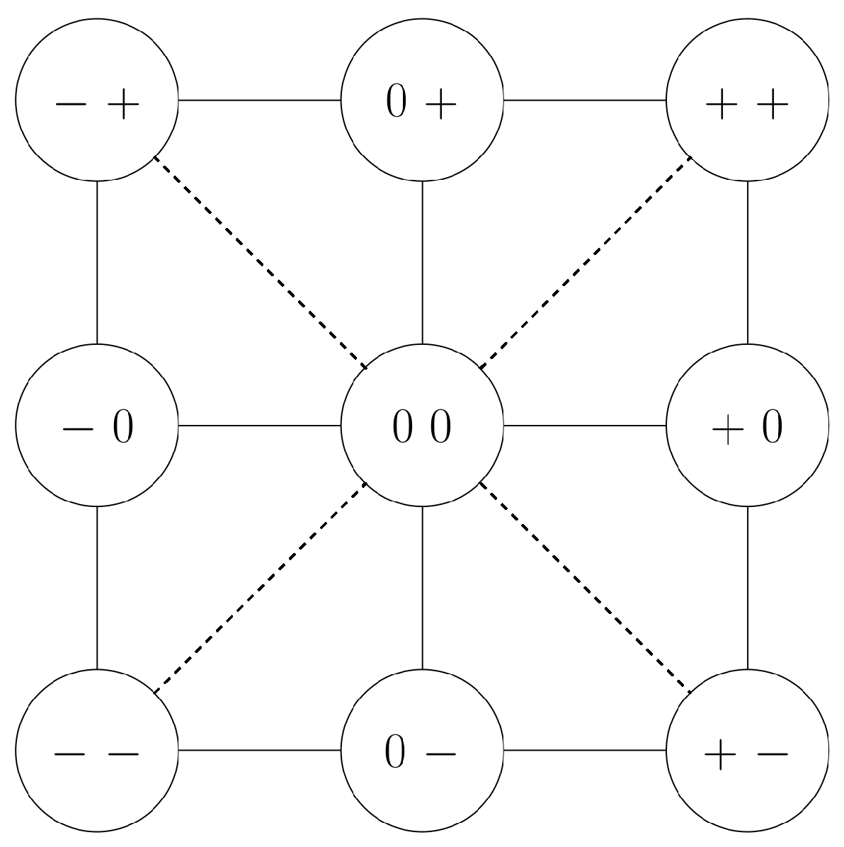
Figure 2.
Conditional Neighbourhood Diagramm (CND) of
. Given continuous observation, it is impossible to transition from moving towards the other agent to moving away from it without passing through the 0-state. Hence, whereas + and − always described intervals in time, 0 states can be of infisitinimal length. Also, note that due to the original formulation [
15], there are no direct transitions in the CND between some of the states that, at a first glance, appear to be adjacent (e.g.,
and
).
The other version of the calculus used in our models, called QTC Double-Cross (
) for 2D movement, extends the previous one to include also the side the two points move to,
i.e., left, right, or straight, and the minimum absolute angle of
k, again with respect to the reference line connecting them (see
Figure 1a).
Figure 1b shows an example human-robot interaction in a corridor, encoded in
. In addition to the 3-tuple
of
, the relations
are considered, where each element can assume any of the values
as follows:
- (q4)
movement of
k with respect to
− : k is moving to the left side of
0 : k is moving along
+ : k is moving to the right side of
- (q5)
movement of l with respect to : as above, but swapping k and l
- (q6)
minimum absolute angle of
k,
with respect to
− :
0 :
+ :
Similar to
we also use the simplified version of
,
. For simplicity we will from here on refer to the simplified versions of QTC,
i.e.,
and
[
15], as
and
respectively. This simplified version inherits from
the ability to model if the agents are moving
apart or
towards each other or are
stable with respect to the last position and in addition is also able to model to which side of the connecting line the agents are moving. The resulting 4-tuple
representing the state set
, has
states, and
legal transitions as defined in the corresponding CND [
41], see
Figure 3.
These are the original definitions of the two used QTC variants which can be used in our computational model to identify HRSI encounters as shown in previous work [
13]. To model distance however, we need both,
and
, in one unified model. As shown in [
12],
and
can be combined using hand crafted and simplified state chains and transitions to represent and reason about HRSIs. In the following section, however, we formalise and automatise this process, ultimately enabling us to use real world data to learn the transitions between the two variants of QTC instead of predefining them
manually.
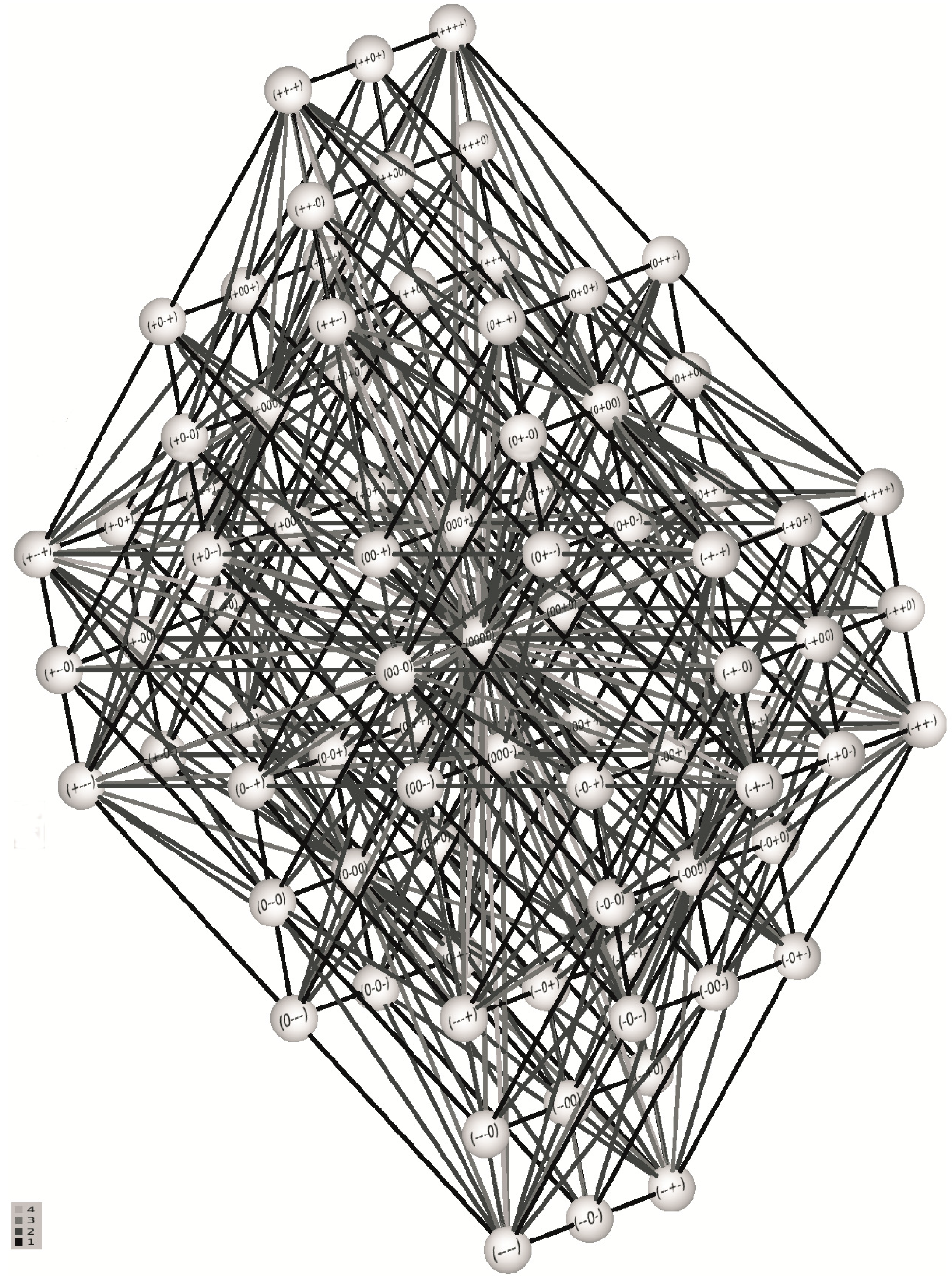
Figure 3.
CND of the simplified
(image source [
41]). Note that, similar to the CND for
, due to the original formulation of CNDs, there are no direct transitions between some of the states that at first glance look adjacent, e.g.,
and
.
Figure 3.
CND of the simplified
(image source [
41]). Note that, similar to the CND for
, due to the original formulation of CNDs, there are no direct transitions between some of the states that at first glance look adjacent, e.g.,
and
.
3.2. Combining and
As mentioned, one of the aims of the proposed computational model is the combination of the 1D representation
, used when the two agents are far apart, and the 2D representation
, used when the agents are in close vicinity to one another. To achieve this combination via the implicit modelling of the distance threshold used and the resulting simplification of QTC state chains for HRSI when encapsulated in our probabilistic framework, we propose the combination of
and
referring to it as
. The combined variants are
and
which results in
, from here on referred to as
for simplicity. This proposed model is in principal able to switch between the fine and coarse version of QTC at will, but for the presented work we will use distance thresholds to trigger the switching. These thresholds could be social distances like the previously mentioned area of far phase personal space and close phase social space as defined by Hall [
8] but could also be any other distance value. Since the actual quantitative distance threshold used is not explicitly included in the
tuple, it will be modelled implicitly via the transition between the two enclosed variants.
The set of possible states for
is a simple unification of the fused QTC variants. In the presented case the integrated
states are defined as:
with
states.
The transitions of
include the unification of the transitions of
and
–as specified in the corresponding CNDs (see
Figure 2 and
Figure 3)–but also the transitions from
to
:
and from
to
:
, respectively. This leads to the definition of
transitions as:
To preserve the characteristics and benefits of the underlying calculus
and
are simply regarded as an increase or decrease in granularity,
i.e., switching from 1D to 2D or vice-versa. As a result there are two different types of transitions:
Pseudo self-transitions where the values of do not change, plus all possible combinations for the 2-tuple : , e.g., or .
Legal transitions, plus all possible combinations for the 2-tuple : , e.g., or .
Resulting into:
transitions between the two QTC variants. This leads to a total number of
transitions of:
These transitions depend on the previous and current Euclidean distance of the two points
and the threshold
representing an arbitrary distance threshold:
These transitions, distances, and threshold play a vital role in our probabilistic representation of which will be described in the following section.
4. Probabilistic Model of State Chains
After introducing our model of
in
Section 3, we will describe a probabilistic model of
state chains in the following. This probabilistic representation is able to learn QTC state chains and the transition probabilities between the states from observed trajectories of human and robot, using the distance threshold
to switch between the two QTC variants during training. This model is later on used as a classifier to compare different encounters and to make assumptions about the quality of the representation. This representation is able to compensate for illegal transitions and shall also be used in future work as a knowledge base of previous encounters to classify and predict new interactions.
In previous work, we proposed a probabilistic model of state chains, using a Markov Model and
to analyse HRSI [
11]. This first approach has been taken a step further and evolved into a Hidden Markov Model (HMM) representation of
[
13]. This enables us to represent actual sensor data by allowing for uncertainty in the recognition process. With this approach, we are able to reliably classify different HRSI encounters, e.g., head-on (see
Figure 4) and overtake–where the human is overtaking the robot while both are trying to reach the same goal–scenarios, and show in
Section 6 that the QTC-based representations of these scenarios are significantly different from each other.
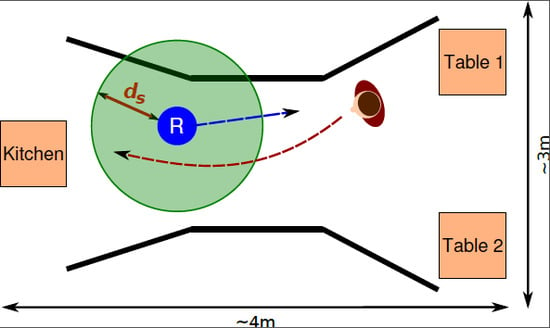
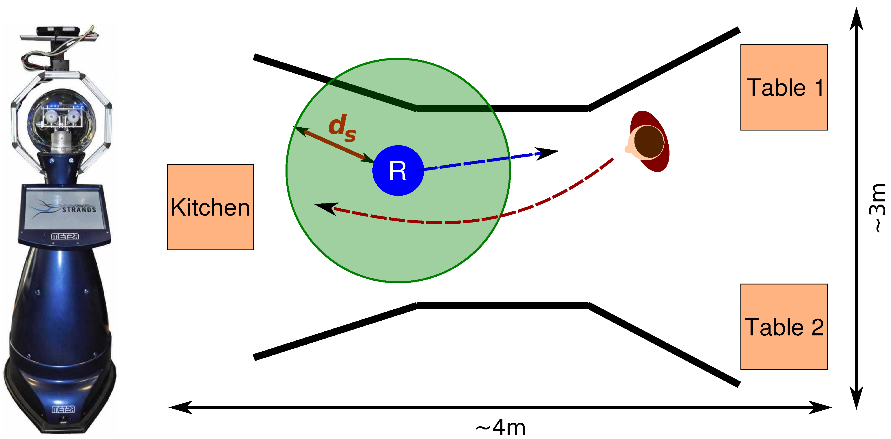
Figure 4.
Left: Robot. Hight: 1.72 m, diameter: ∼ 61 cm. Right: Head-on encounter. Robot (“R”) tries to reach a table while the human (reddish figure) is trying to reach the kitchen. Experimental set-up: kitchen on the left and two tables on the right. Black lines represent the corridor. Circle around robot represents a possible distance threshold .
To be able to represent distance for future extensions of the HMM as a generative model, to highlight events in close vicinity to the human, and to create a more concise and tractable model, we propose the probabilistic representation of
state chains, using a similar approach as in [
13]. We are now modelling the proposed
together with
and
which allows to dynamically switch between the two combined variants or to use the two pure forms of the calculus. This results in extended transition and emission probability matrices for
(see
Figure 5, showing the transition probability matrix) which incorporate not only
and
, but also the transitional states defined by
.
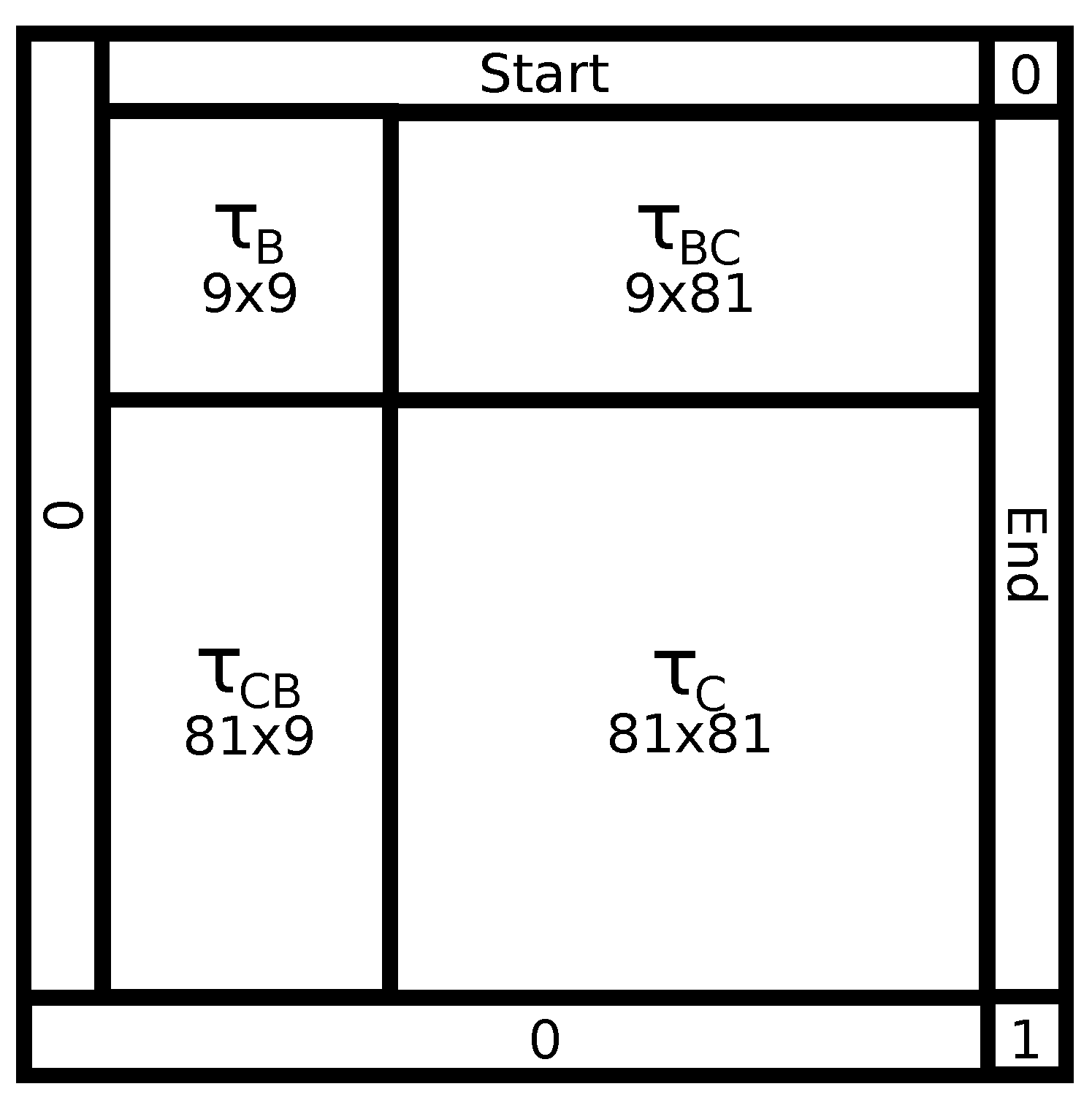
Figure 5.
The HMM transition matrix
for
as described in Equations (
2) and (
3).
Figure 5.
The HMM transition matrix
for
as described in Equations (
2) and (
3).
Similar to the HMM based representation described in [
13], we have initially modelled the “correct” emissions, e.g.,
actually emits
, to occur with
probability and to allow the model to account for detection errors with
. Our HMM contains
legal transitions stemming from
and the transitions from and to the start and end state, respectively (see
Figure 5).
To represent different HRSI behaviours, the HMM needs to be trained from the actual observed data (see
Figure 6, showing an example of a trained state chain using pure
). For each different behaviour to be represented, a separate HMM is trained, using Baum-Welch training [
42] (Expectation Maximisation) to obtain the appropriate transition and emission probabilities for the respective behaviour. In the initial pre-training model, the transitions that are
valid, according to the CNDs for
and
and our
definition for transitions between the two, are modelled as equally probable (uniform distribution). We allow for pseudo-transitions with a probability of
to overcome the problem of a lack of sufficient amounts of training data and unobserved transitions therein. To create the training set we have to transform the recorded data to
state chains that include the Euclidean distance between
k and
l and define a threshold
at which we want to transition from
to
and vice-versa (setting
results in a pure
model and setting
results in pure
model–identical to the definition in [
13] for full backwards compatibility). Of course, the actual values for
can be anything from being manually defined, taken from observation, or being a probabilistic representation of a range of distances at which to transition from one QTC variant to the other. For the sake of our evaluation we are showing a range of possible values for
in
Section 6 to find suitable candidates.
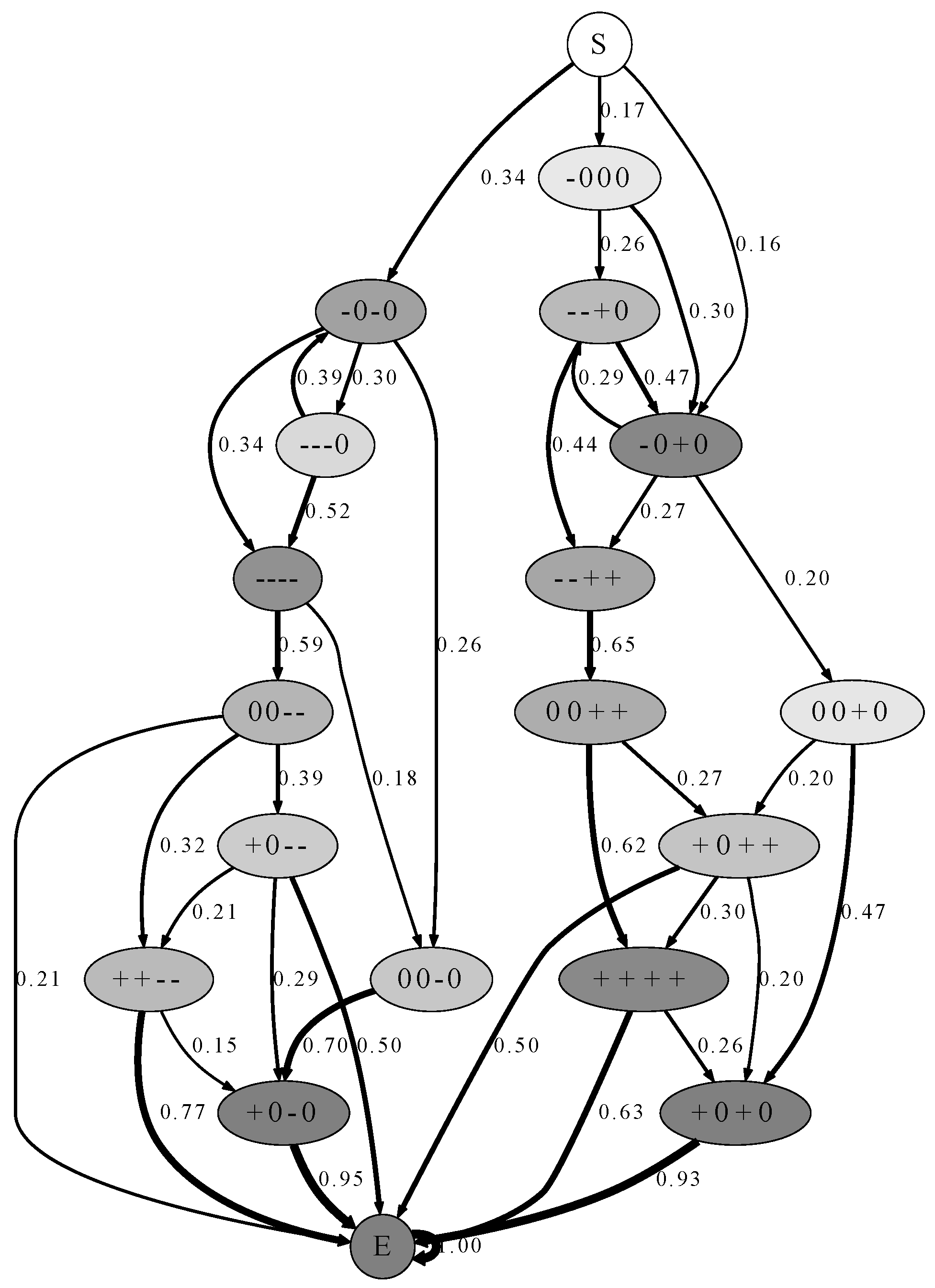
Figure 6.
states for pass-by situations created by the HMM representation. Edge width represents the transition probability. The colour of the nodes represents the a-priori probability of that specific state (from white = 0.0, e.g., “S”, to dark grey = 1.0, e.g., “E”). All transition probabilities below 0.15 have been pruned from the graph, only highlighting the most probable paths within our model. Due to the pruning, the transition probabilities in the graph do not sum up to 1.0.
To create a state chain similar to the exemplary one shown in
Figure 7, the values for the side movement
of the
representation are simply omitted if
and the remaining
2-tuple for the 1D movement will be represented by the
part of the transition matrix. If the distance crosses the threshold, it will be represented by one of the
or
transitions. The full 2D representation of
is used in the remainder of the cases. Afterwards, all distance values are removed from the representation because the QTC state chain now implicitly models
, and similar adjacent states are collapsed to create a valid QTC representation (see
Figure 7 for a conceptual state chain). This enables us to model distance via the transition between the QTC variants, while still using the pure forms of the included calculi in the remainder of the cases, preserving the functionality presented in [
13], which will be shown in
Section 6.
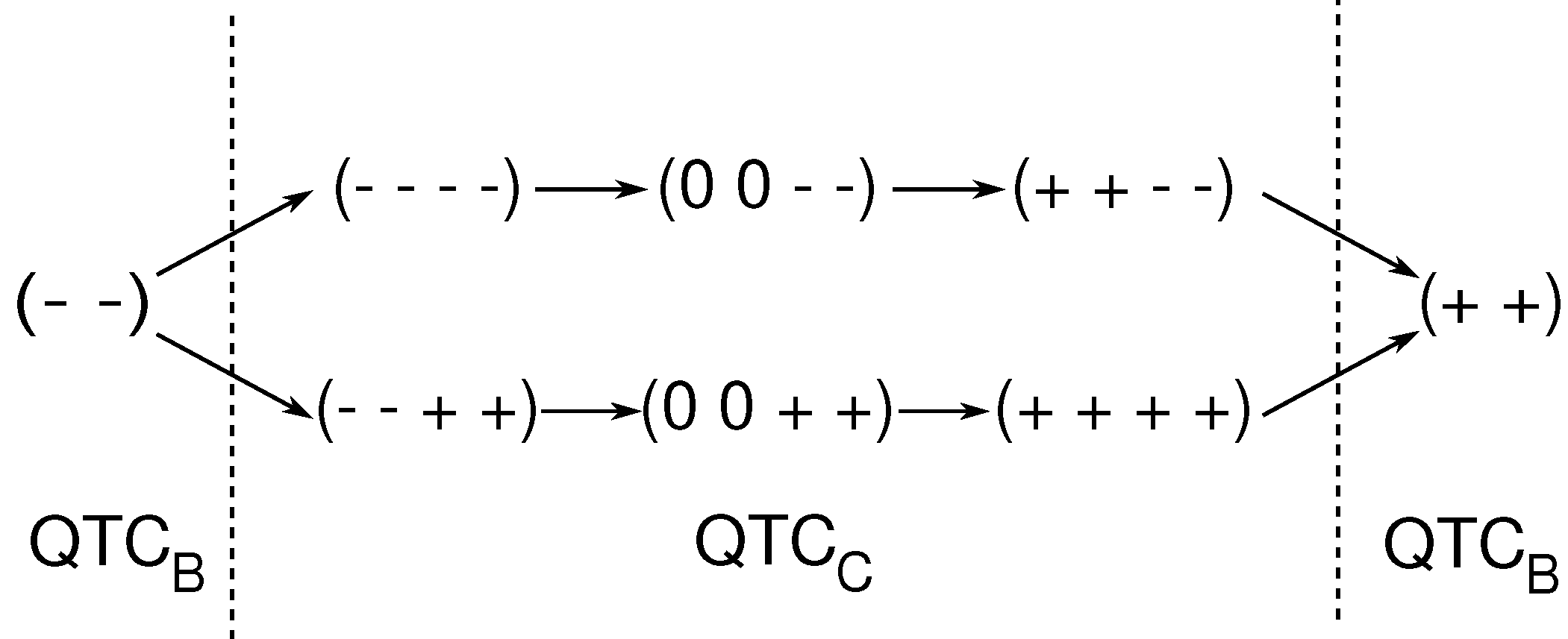
Figure 7.
Conceptual temporal sequence of for a head-on encounter. From left to right: approach, pass-by on the left or right side, moving away. Dashed lines represent instants where the distance threshold is crossed.
Figure 7.
Conceptual temporal sequence of for a head-on encounter. From left to right: approach, pass-by on the left or right side, moving away. Dashed lines represent instants where the distance threshold is crossed.
5. Experiments
To evaluate the soundness and representational capabilities of our probabilistic model of HRSI using QTC, particularly
, state chains, we train our HMM representation using real-world data from two experiments. These HMMs are then employed as classifiers to generate a comparative measurement enabling us to make assumptions about the quality of the model and the distance thresholds
. The two experiments both investigate the movement of two agents in confined shared spaces. The first experiment, later referred to as “Lincoln experiment”, was originally described in our previous work on QTC [
13] and features a mobile service robot and a human naïve to the goal of the experiment. The tasks were designed around a hypothetical restaurant scenario eliciting incidental and spontaneous interactions between human and robot.
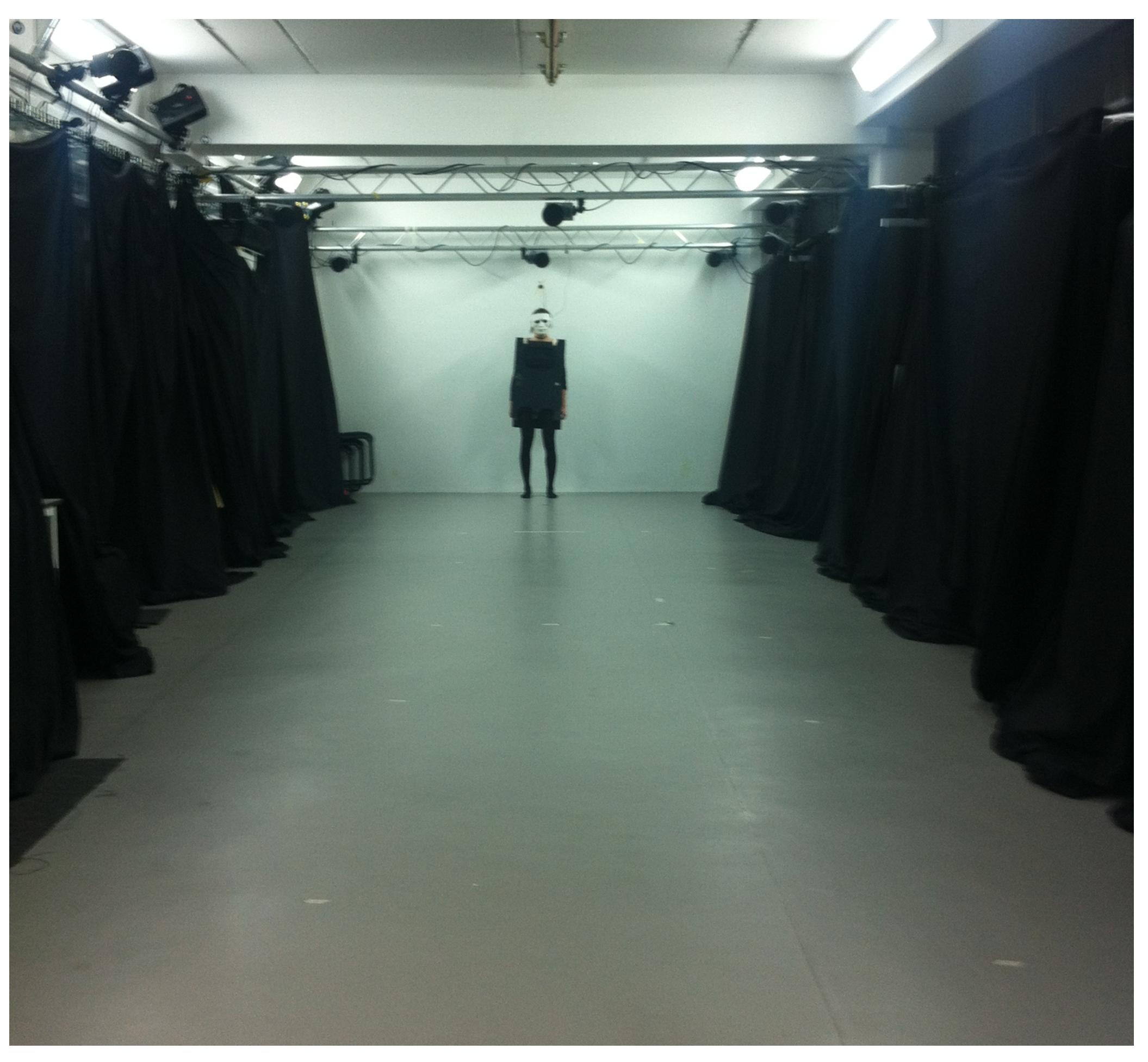
The second experiment, later referred to as the “Bristol experiment”, features two agents (both human) passing each other in a two meter wide corridor. One of the two (the experimenter) was dressed up as a “robot”, masking her body shape, and her face and eyes were hidden behind goggles and a face mask (see
Figure 8). This “fake robot” received automated instructions on movement direction and collision avoidance strategy via headphones. Similar to the “Lincoln experiment”, the other person was a participant naïve to the goal of the experiments, but has been given explicit instructions to cross the corridor with as little veering as possible, but without colliding with the oncoming agent. This second experiment does not feature a real robot but, yields similar results using our model, as can be seen in
Section 6. Both experiments feature two agents interacting with each other in a confined shared space and are well suited to demonstrate the representational capabilities of our approach, showing how the approach can be effectively generalised or extended to other forms of spatial interaction.
Figure 8.
The “Bristol Experiment” set-up. Corridor from the participants perspective before the start of a trial. Middle: experimenter dressed as “robot”. The visual marker was attached to the wall behind the “robot” above her head.
Figure 8.
The “Bristol Experiment” set-up. Corridor from the participants perspective before the start of a trial. Middle: experimenter dressed as “robot”. The visual marker was attached to the wall behind the “robot” above her head.
In the following sections we will describe the general aims and outlines of the experiments used. This is meant to paint the bigger picture of the underlying assumptions and behaviours of the robot/experimenter during the interactions and to explain some of the conditions we compared in our evaluation. Both experiments investigated different aspects of HRSI and spatial interaction in general, which created data well suited for our analysis of the presented probabilistic model utilising and to investigate appropriate distance thresholds .
5.1. “Lincoln Experiment”
This section presents a brief overview of the “Lincoln experiment” set-up and tasks. Note, the original aim of the experiment, besides the investigation of HRSI using an autonomous robot in general, was finding hesitation signals in HRSI [
43], hence the choice of conditions.
5.1.1. Experiment Design
In this experiment the participants were put into a hypothetical restaurant scenario together with a human-size robot (see
Figure 4). The experiment was situated in a large motion capture lab surrounded by 12 motion capture cameras (see
Figure 9), tracking the
coordinates of human and robot with a rate of 50 Hz and an approximate error of 1.5 mm∼2.5 mm. The physical set-up itself was comprised of two large boxes (resembling tables) and a bar stool (resembling a kitchen counter). The tables and the kitchen counter were on different sides of the room and connected via a ∼2.7 m long and ∼1.6 m wide artificial corridor to elicit close encounters between the two agents while still being able to reliably track their positions (see
Figure 4). The length is just the length of the actual corridor, whereas the complete set-up was longer due to the added tables and kitchen counter plus some space for the robot and human to turn. The width is taken from the narrowest point. At the ends, the corridor widens to ∼ 2.2 m to give more room for the robot and human to navigate as can be seen in
Figure 4. The evaluation however will only regard interactions in this specified corridor. For this experiment we had 14 participants (10 male, 4 female) who interacted with the robot for 6 minutes each. All of the participants were employees or students at the university and 9 of them have a computer science background; out of these 9 participants only 2 had worked with robots before. The robot and human were fitted with motion capture markers to track their
coordinates for the QTC representation–
Figure 10 shows an example of recorded trajectories (the raw data set containing the recorded motion capture sequences is publicly available on our git repository [
44]).
The robot was programmed to move autonomously back and forth between the two sides of the artificial corridor (kitchen and tables), using a state-of-the-art planner [
45,
46]. Two different behaviours were implemented,
i.e.,
adaptive and
non-adaptive velocity control, which were switched at random (
) upon the robot’s arrival at the kitchen. The adaptive velocity control gradually slowed down the robot, when entering the close phase of the social space [
8], until it came to a complete stand still before entering the personal space [
8] of the participant. The non-adaptive velocity control ignored the human even as an obstacle (apart from an emergency stop when the two interactants were too close, approx. <0.4 m, to prevent injuries), trying to follow the shortest path to the goal, only regarding static obstacles. This might have yielded invalid paths due to the human blocking it, but led to the desired robot behaviour of not respecting the humans personal space. We chose to use these two distinct behaviours because they mainly differ in the speed of the robot and the distance it keeps to the human. Hence, they produce very similar, almost straight trajectories which allowed us to investigate the effect of distance and speed on the interaction while the participant was still able to reliably infer the robot’s goal. As mentioned above, this was necessary to find hesitation signals [
43].
Figure 9.
The “Lincoln experiment” set-up showing the robot, the motion capture cameras, the artificial corridor, and the “tables” and “kitchen counter”. The shown set-up elicits close encounters between human and robot in a confined shared space to investigate their interaction.
Figure 9.
The “Lincoln experiment” set-up showing the robot, the motion capture cameras, the artificial corridor, and the “tables” and “kitchen counter”. The shown set-up elicits close encounters between human and robot in a confined shared space to investigate their interaction.
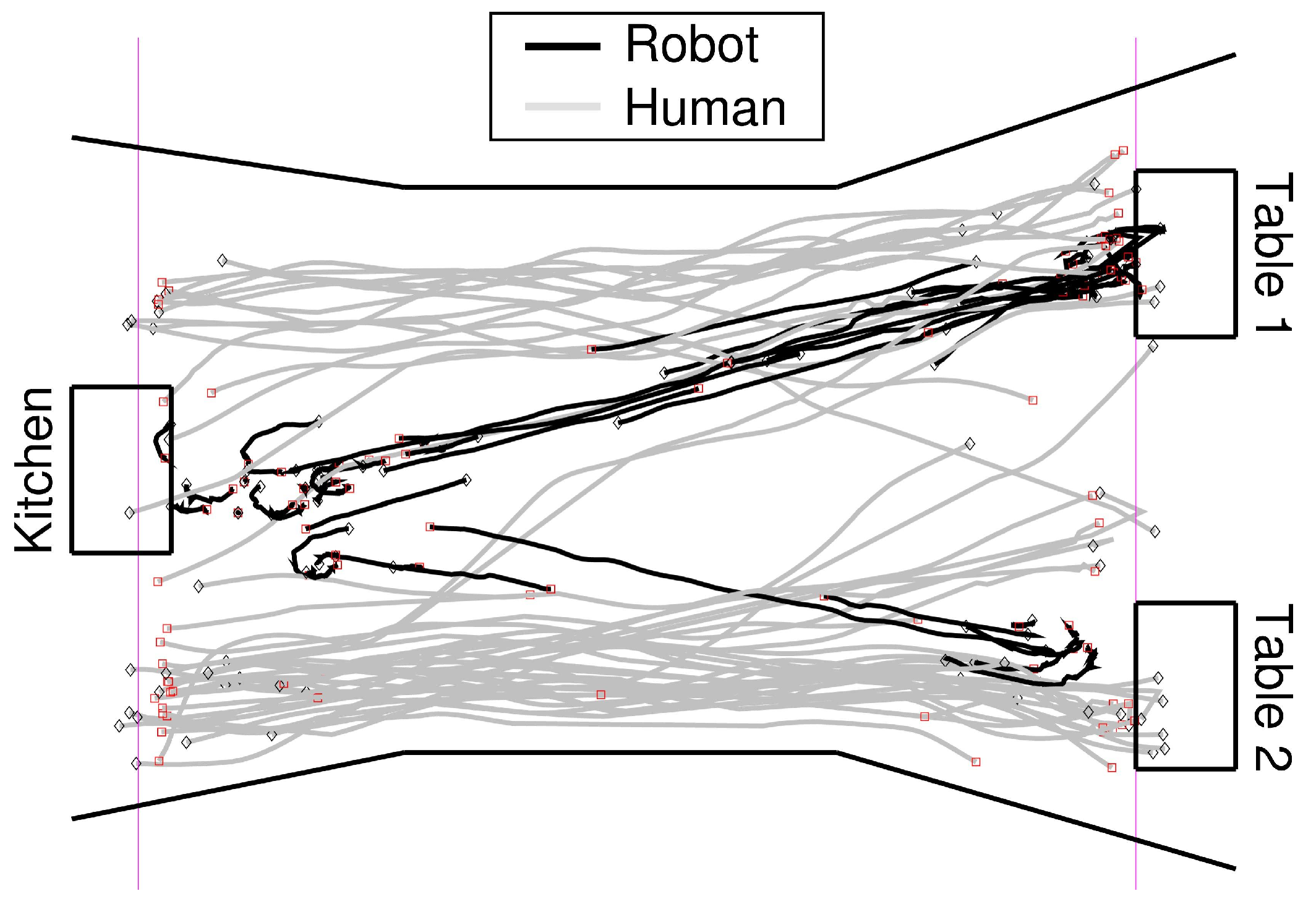
Figure 10.
The recorded trajectories of one of the participants (grey = human, black = robot). The rough position of the corridor walls and the furniture is also depicted. The pink lines on either side show the cut-off lines for the evaluation. The robots trajectories were not bound to the cut-off lines but to the humans trajectories timestamps. The humans trajectories themselves might not end at the cut-off line but before due to those regions being on the outside limits of the tracking region, causing the loss of markers by the tracking system.
Before the actual interaction, the human participant was told to play the role of a waiter together with a robotic co-worker. This scenario allowed to create a natural form of pass-by interaction (see
Figure 4 and
Figure 1b) between human and robot by sending the participants from the kitchen counter to the tables and back to deliver drinks, while at the same time the robot was behaving in the described way. This task only occasionally resulted in encounters between human and robot but due to the incidental nature of these encounters and the fact that the participants were trying to reach their goal as efficiently as possible, we hoped to achieve a more natural and instantaneous participant reaction.
5.2. “Bristol Experiment”
In the following, we will give a quick overview of the “Bristol experiment” set-up and tasks. Besides investigating general HRSI concepts, the main aim of the experiment was to investigate the impact and dynamics of different visual signal types to inform an on-coming agent of the direction of intended avoidance manoeuvres in an artificial agent in HRSI, hence the comparatively complex set-up of conditions. For the purpose of the QTC analysis presented, however, we will just look at a specific set of conditions out of the ones mentioned in the experiment description.
5.2.1. Experiment Design
In this experiment, 20 participants (age range 19–45 years with a mean age of 24.35) were asked to pass an on-coming “robotic” agent (as mentioned above, a human dressed as a robot, from now on referred to as “robot”) in a wide corridor. The corridor was placed in the Bristol Vision Institute (BVI) vision and movement laboratory, equipped with 12 Qualisys 3D-motion capture cameras. The set-up allows to track movement of motion capture markers attached to the participants and the robot in
-coordinates over an area of 12 m (long) × 2 m (wide) × 2 m (high) (see
Figure 8) with a frequency of 100 Hz and an approximate error of 1 mm.
Participants were asked to cross the laboratory toward a target attached to the centre of the back wall (and visible at the beginning of each trial at the wall above the head of the “robot”) as directly as possible, without colliding with the on-coming “robot”. At the same time, the “robot” would cross the laboratory in the opposite direction, thus directly head-on to the participant. In 2/3 of the conditions, the “robot” would initiate an automated “avoidance behaviour” to the left or right of the participant that could be either accompanied by a visual signal indicating the direction of the avoidance manoeuvre or be unaccompanied by visual signals (see
Figure 11 for the type of signals). Note that if neither robot nor participant were to start an avoidance manoeuvre, they would collide with each other approximately midway through the laboratory.
The robot, dressed in a black long-sleeved T-shirt and black leggings, was wearing a “robot suit” comprising of two black cardboard boards (71 cm high × 46 cm wide) tied together over the agent’s shoulders on either side with belts (see
Figure 8). The suit was intended to mask body signals (e.g., shoulder movement) usually sent by humans during walking. To also obscure the “robots” facial features and eye gaze, the robot further wore a blank white mask with interiorly attached sunglasses.
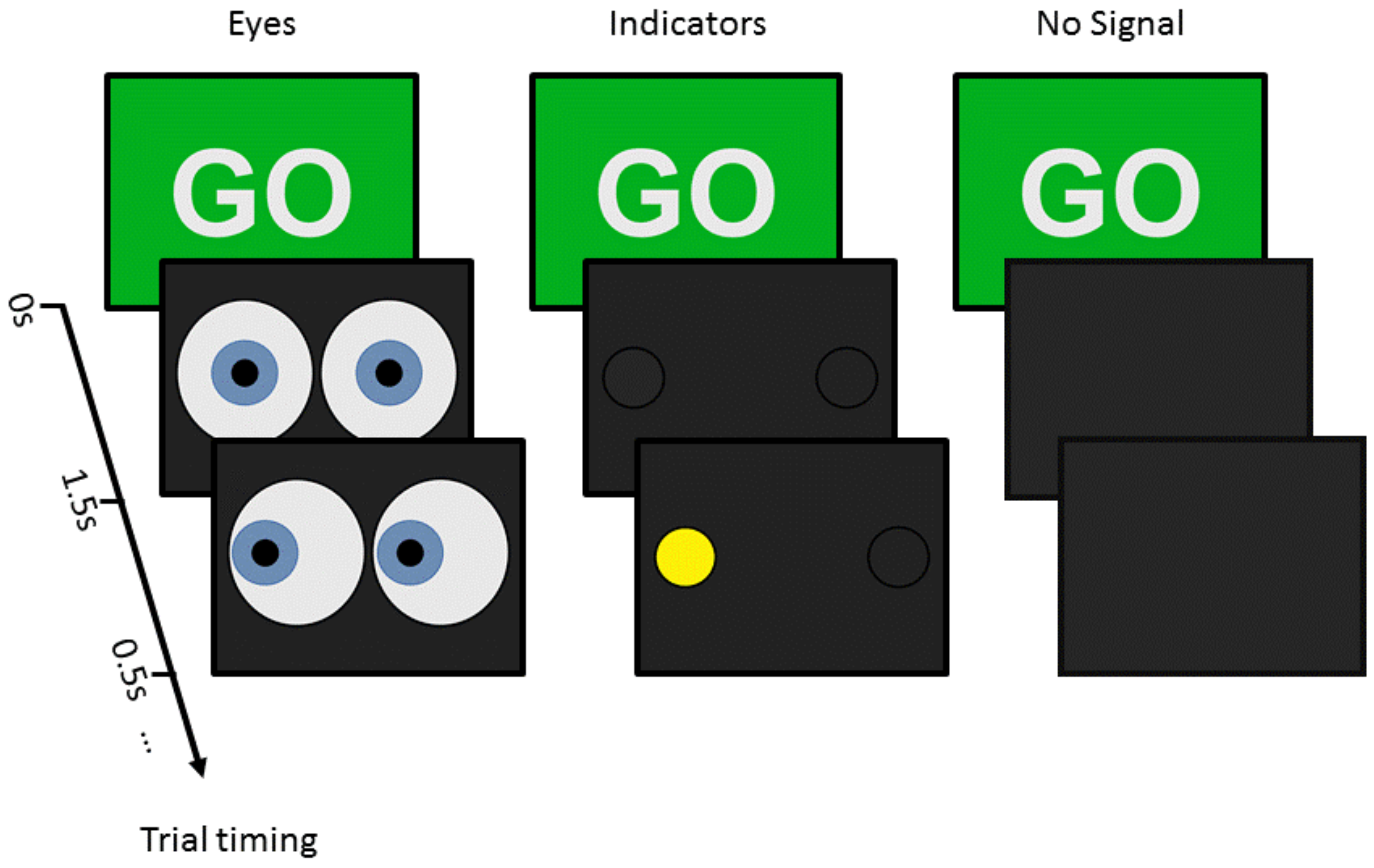
A Nexus 10 Tablet (26 cm × 18 cm) was positioned on the cardboard suit at chest height to display a “go” signal at the beginning of each trial to inform the participant that they should start walking. The go signal was followed 1.5 s later by the onset of visual signals (cartoon eyes, indicators, or a blank screen as “No signal”). With exception of the “no signal”, these visual signals stayed unchanged in a third of the trials, and in the other 2 thirds of trials, they would change 0.5 s later to signal the direction in which the robot would try to circumvent the participant (the cartoon eyes would change from straight ahead to left or right, the indicators would start flashing left or right with a flash frequency of 2 Hz). Note that no deception was used; i.e., if the robot indicated a direction to the left or right, it would always move in this direction. However, if the robot did not visually indicate a direction, it would still move to the left or right in two thirds of trials. Only in the remaining trials, the robot would keep on walking straight, thus forcing the participant to avoid collision by actively circumventing the robot.
Figure 11.
Examples of visual signals sent by the “robot” agent. Visual signal onset occurred 1.5 s after the “go” signal encouraging the participant to start walking. 500 ms after the signal onset, signals could either then change to indicate a clear direction in which the robot would avoid the participant or remain uninformative with respect to the direction of movement of the robot.
The actual/physical onset of the robot’s avoidance manoeuvres could start 700 ms before the visual directional signal was given (early), at the time of the visual direction signal (middle), or 700 ms after the onset of the visual direction signal (late). These three conditions will later on be referred to as early, middle, or late, respectively.
In the following we will focus on the trajectories taken by both agents in this confined shared space and compare some of the conditions used.
5.3. Evaluation
The aim of the evaluation is to test the descriptive quality of the created probabilistic sequential model utilising QTC state chains in general, to evaluate possible distance thresholds or ranges of thresholds to be incorporated into the model, and to learn appropriate transitions between the QTC variants for our model. To this end, the models created from the recorded trajectories are employed as classifiers to generate comparative measurements, allowing to make statements about the representational quality of the model itself. These classifiers use a range of distance thresholds to find those values appropriate for the switch from to and vice-versa. The goal of this evaluation therefore is not to compare the quality or appropriateness of the different QTC variants but their combination with our probabilistic model to represent HRSI. Hence, classification is not only an important application for our model but we are also using it as a tool to create a comparative measurement for evaluation.
To quickly recapitulate, the different QTC variants we are using in the following are: (i) -1D: represents approach, moving away, or being stable in relation to the last position; (ii) -2D: in addition to , also includes to which side the agents are moving, left of, right of, or along the connecting line; (iii) -1D/2D: the combination of both according to the distance of the two agents, (1D) when far apart and (2D) when close. The 0 states mentioned in the following are therefore instances in time when the agent was stable in its 1-dimensional and/or 2-dimensional movement.
The data of both experiments will be used equally for our evaluation. However, due to the different nature of the investigated effects and signals, and the resulting different set-ups used, there will be slight differences in the evaluation process and therefore it will be split in two parts according to the experiments. The used model on the other hand, will be the same for both experiments to show its generalisability. In the following we will present the used evaluation procedures for each study.
Lincoln Experiment We defined two virtual cut-off lines on either side of the corridor (see
Figure 10) to separate the trajectories into trials and because we only want to investigate close encounters between human and robot and therefore just used trajectories inside the corridor. Out of these trajectories, we manually selected 71 head-on and 87 overtaking encounters and employed two forms of noise reduction on the recorded data. The actual trajectories were smoothed by averaging over the
coordinates for 0.1 s, 0.2 s, and 0.3 s. The
z coordinate is not represented in QTC. To determine 0 QTC states–one or both agents move along
or along the two perpendicular lines (see
Figure 1)–we used three different quantisation thresholds: 1 cm, 5 cm, and 10 cm, respectively. Only if the movement of one or both of the agents exceeded these thresholds it was interpreted as a − or + QTC state. This smoothing and thresholding is necessary when dealing with discrete sensor data which otherwise would most likely never produce 0 states due to sensor noise.
To find appropriate distance thresholds for , we evaluated distances on a scale from pure (40 cm) to pure (3 m), in 10 cm steps. The m threshold represents pure because the robot and human are represented by their centre points, therefore, it is impossible for them to get closer than 40 cm . On the other hand, the m threshold represents pure because the corridor was only ∼ 2.7 m long.
We evaluated the head-on vs. overtake, passing on the left vs. right, and adaptive vs. non-adaptive velocity conditions.
Bristol Experiment Following a similar approach as described above, we split the recorded data into separate trials, each containing one interaction between the “robot” and the participant. To reduce noise caused by minute movements before the beginning and after the end of a trial, we removed data points from before the start and after the end of the individual trial by defining cut off lines on either end of the corridor, only investigating interactions in between those boundaries. Visual inspection for missing data points and tracking errors yielded 154 erroneous datasets out of the 1439 trials in total and were excluded from the evaluation. Similar to the Lincoln data set, we applied three different smoothing levels 0.00 s, 0.02 s, and 0.03 s. We also used four different quantisation levels, 0.0 cm, 0.1 cm, 0.5 cm, and 1 cm, to generate QTC 0-states (due to the higher recording frequency of 100 Hz the smoothing and quantisation values are lower than for the Lincoln experiment). Unlike the “Lincoln experiment”, one of the smoothing and quantisation combinations, i.e., 0.0 s and 0.0 cm, represents unsmoothed and unquantised data. This was possible due to a higher recording frequency and a less noisy motion capture system.
We evaluated distances on a scale from pure (40 cm) to 3 m, in 10 cm steps. To stay in line with our first experiment, we evaluated distances of up to 3 m but since the corridor had a length of 12 m, we also added a pure representation () for comparison.
In this experiment we did not investigate overtaking scenarios as those were not part of the experimental design. We evaluated passing on the left vs. right and indicator vs. no indicator separated according to their timing condition (i.e., early, middle, late), and early vs. late regardless of any other condition.
Statistical Evaluation To generate the mentioned comparative measurement to evaluate the meaningfulness of the representation, we used our previously described HMM based representation as a classifier comparing different conditions. With this measurement, we are later on able to make assumptions about the quality and representational capabilities of the model itself.
For the classification process, we employed k-fold cross validation with , resulting in five iterations with a test set size of 20% of the selected trajectories. This was repeated ten times for the “Lincoln experiment” and 4 times for the “Bristol experiment”–to compensate for possible classification artefacts due to the random nature of the test set generation–resulting in 50 and 20 iterations over the selected trajectories, respectively. The number of repetitions for the “Bristol experiment” is lower due to the higher number of data points and the resulting increase in computation time and decrease in feasibility. Subsequently, a normal distribution was fitted over the classification results to generate the mean and 95% confidence interval and make assumptions about the statistical significance. Being significantly different from the null hypothesis (; ) for the evaluations presented in the following section would therefore imply that our model is expressive enough to represent the encounter it was trained for. This validation procedure was repeated for all smoothing and quantisation combinations.
7. Discussion
In this section we focus on the interpretation of the classification results presented in
Section 6. As described above, employing our probabilistic models as classifiers is used to generate a comparative measure to make assumptions about the quality of the generated representation where significant differences between the two used classes means that our model was able to reliably represent this type of interaction. We are evaluating the general quality of using QTC for the representation of HRSI and investigate the different distances or ranges of distances for the proposed
based model to find suitable regions for the switch between the two variants.
Limitations A possible limitation is that the presented computational model was not evaluated in a dedicated user study but on two data sets from previous experiments. However, a model of HRSI should be able to represent any encounter between a robot and a human in a confined shared space. The two used experiments might not have been explicitly designed to show the performance of the presented approach but provide the type of interactions usually encountered in corridor type situations, which represents a major part of human-aware navigation. Additionally, the instructions given in the “Bristol Experiment”, to cross the corridor with as little veering as possible, might have also influenced the participants behaviour when it comes to keeping the appropriate distances and will therefore also have influence on their experienced comfort and the naturalness of the interaction. However, as we can see from
Figure 15, the left
vs. right conditions yielded similar results in both experiments which indicates that these instructions did not have a significant influence on the participants spatial movement behaviour. Future work, including the integration of this system into an autonomous robot however, will incorporate user studies in a real work environment evaluating not only the performance of the presented model but also of a larger integrated system building upon it.
Our presented probabilistic uses and to determine if the representation should transition from to or vice-versa. This might lead to unwanted behaviour if the distance oscillates around . This has to be overcome for “live” applications, e.g., by incorporating qualitative relations with learned transition probabilities for close and far. For the following discussion, due to the experimental set-up, we can assume that this had no negative effect on the presented data.
A general limitation of QTC is that actual sensor data does not coincide with the constraints of a continuous observation model represented by the CND. In the “Lincoln” data for example we encountered up to 521 illegal transitions which indicates that raw sensor data is not suitable to create QTC state sequences without post-processing. This however, was solved by using our proposed HMM based modelling adhering to the constraints defined in the CND, only producing valid state transitions.
A major limitation is that important HRSI concepts such as speed, acceleration, and distance, are hard to represent using QTC. While regular
is able to represent relative speeds, it is neither possible to represent the velocity nor acceleration of the robot or the human. Therefore, QTC alone is not very well suited to make statements about
comfort,
naturalness, and
sociability, as defined by Kruse
et al. [
9], of a given HRSI encounter. We showed that, using implicit distance modelling is able to enrich QTC with such concepts but many more are missing.
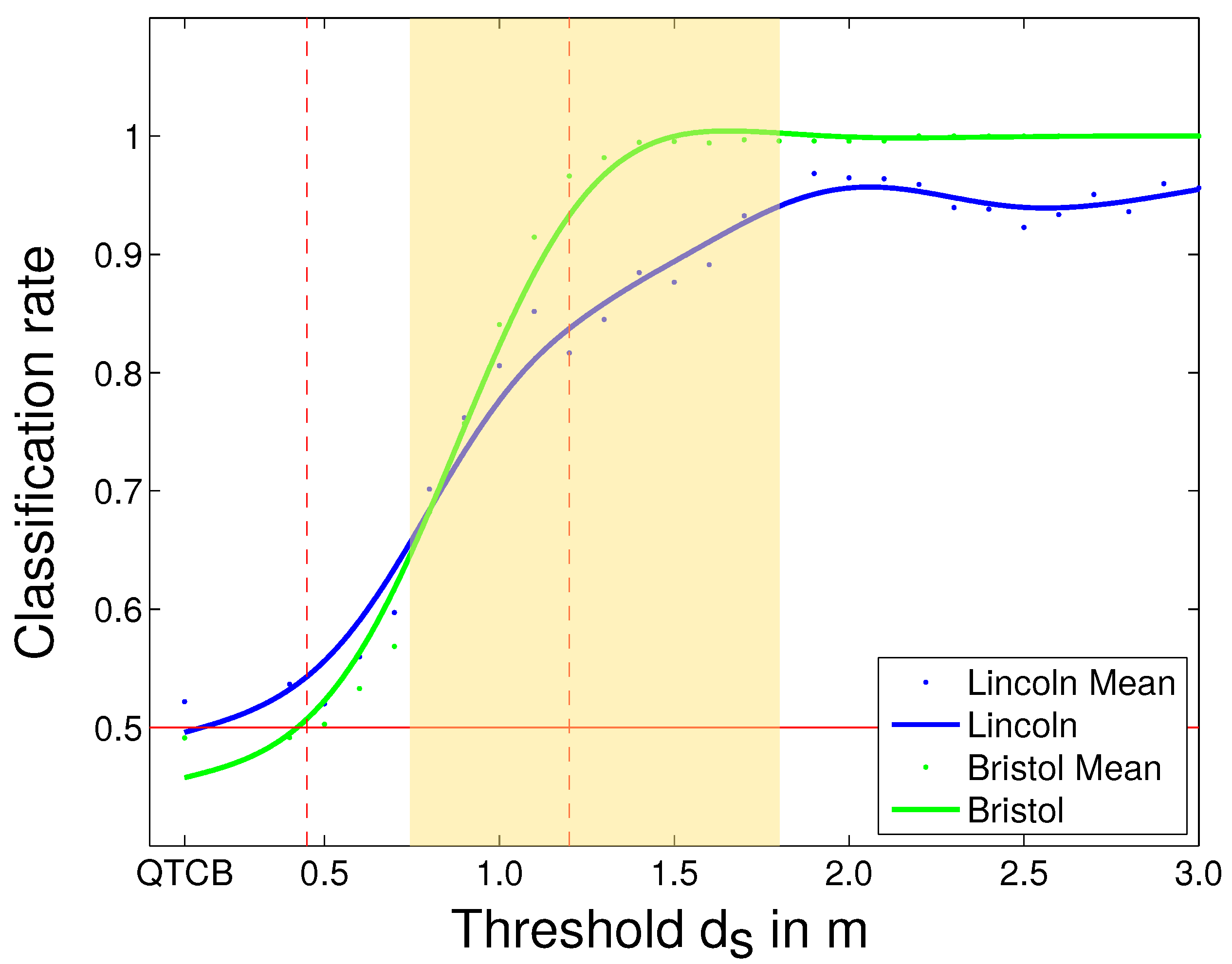
Figure 15.
Comparing “Lincoln” and “Bristol” experiment results: Passing on the left
vs. passing on the right. The blue curve represents the “Lincoln” experiment classification rates using the lowest smoothing values and the green curve represents the unsmoothed classification rate for the “Bristol” experiment, respectively. The curve has been obtained using a smoothing spline [
47] with a
p-value of
. Red line:
, left dashed red line: intimate space [
8], right dashed red line: personal space [
8], yellow area: maximum interval for
transitions. The better results for the “Bristol” experiment can be explained by the larger amount of training data.
Another limitation of QTC is the impossibility to infer which agent executes the actual circumvention action in the head-on scenario. When interpreting the graph in
Figure 6, we are not sure if the human, the robot, or both are circumventing each other. We just know that the human started the action but we do not know if the robot participated or not. This could eventually be countered by using the full
approach including the relative angles. Even then, it might not be possible to make reliable statements about that and it would also complicate the graph and deprive it of some of its generalisation abilities.
Head-on vs. Overtake The presented classification of head-on
vs. overtaking (see
Table 1a) shows that
,
, and
, regardless of the chosen
, are able to reliably classify these two classes. We have seen that there are cases where pure
outperforms pure
. This is not surprising because the main difference of overtaking and head-on lies in the
2-tuple of
,
i.e., both agents move in the same direction, e.g.,
,
vs. both agents are approaching each other
. The 2D
information can therefore be disregarded in most of the cases and only introduces additional noise. This indicates that
would be sufficient to classify head-on and overtaking scenarios but would of course not contain enough information to be used as a generative model or to analyse the interaction.
allows to incorporate the information about which side robot and human should use to pass each other and the distance at which to start circumventing. Additionally,
also allows to disregard information for interactants far apart, only employing the finer grained
where necessary,
i.e., when close to each other. Since all of the found classification results were significantly different from
–the Null Hypothesis (
) for a two class problem–this distance can be freely chosen to represent a meaningful value like Hall’s personal space 1.22 m [
8]. By doing so, we also create a more concise and therefore tractable model as mentioned in our requirements for HRSI modelling.
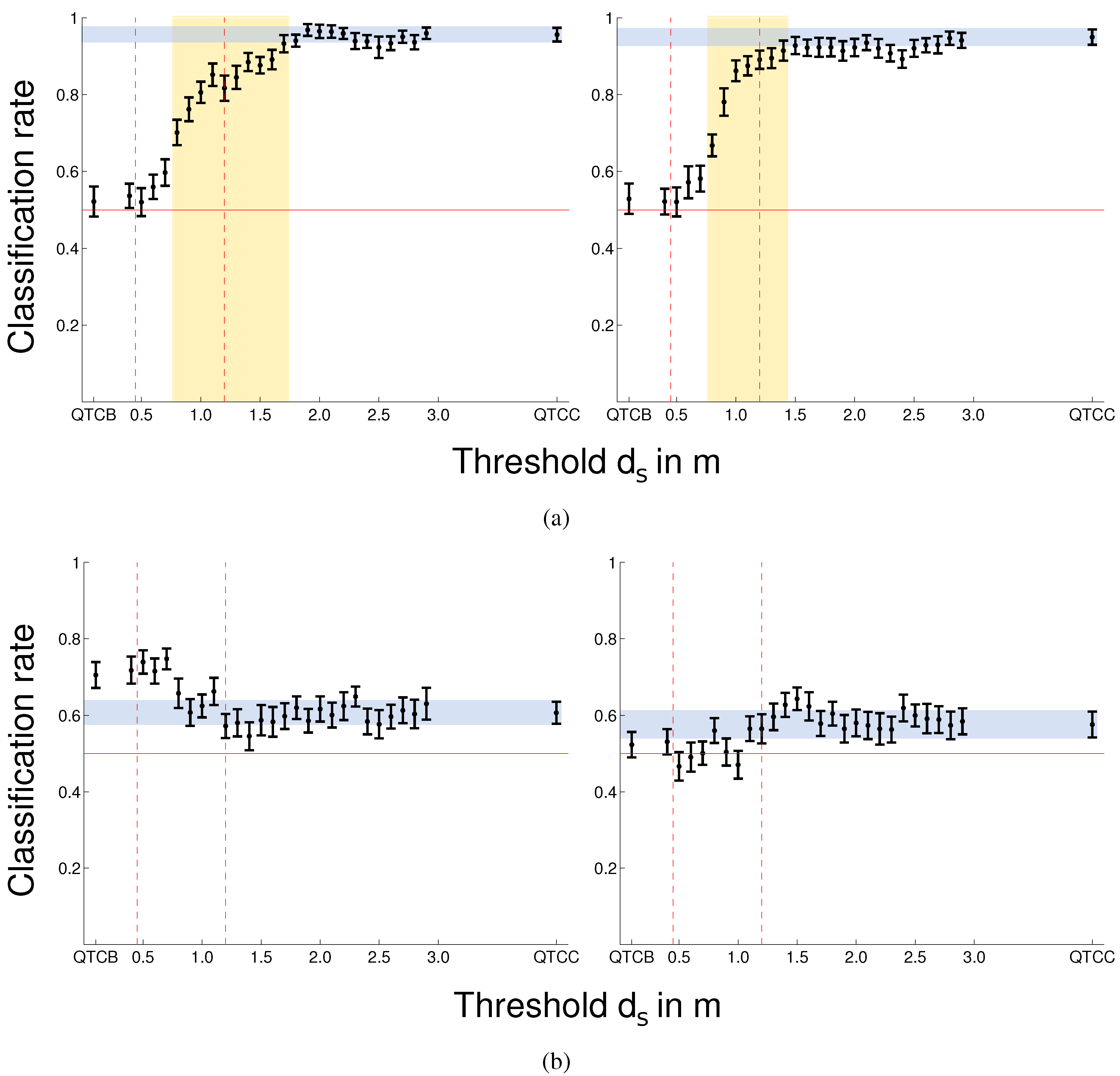
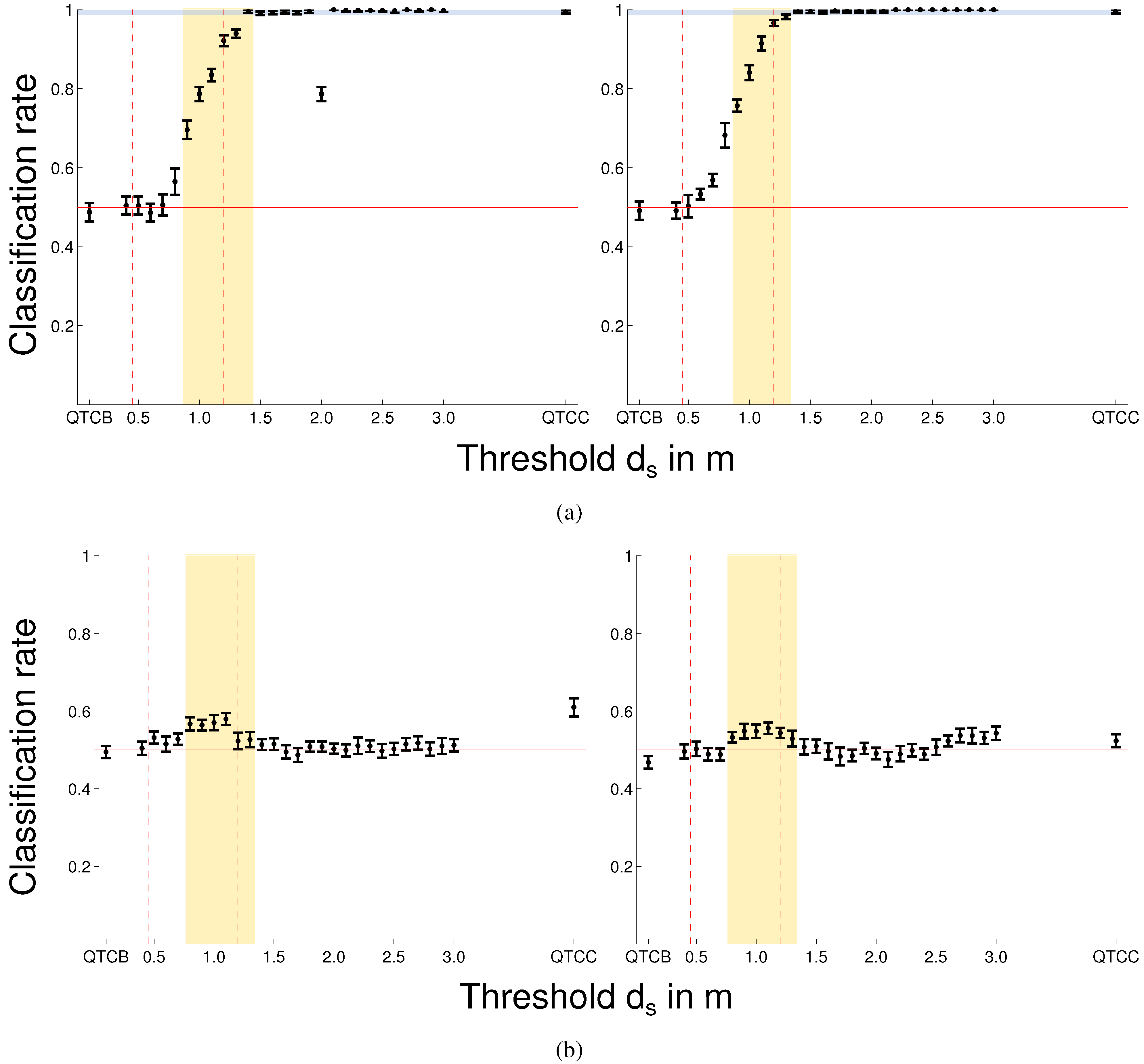
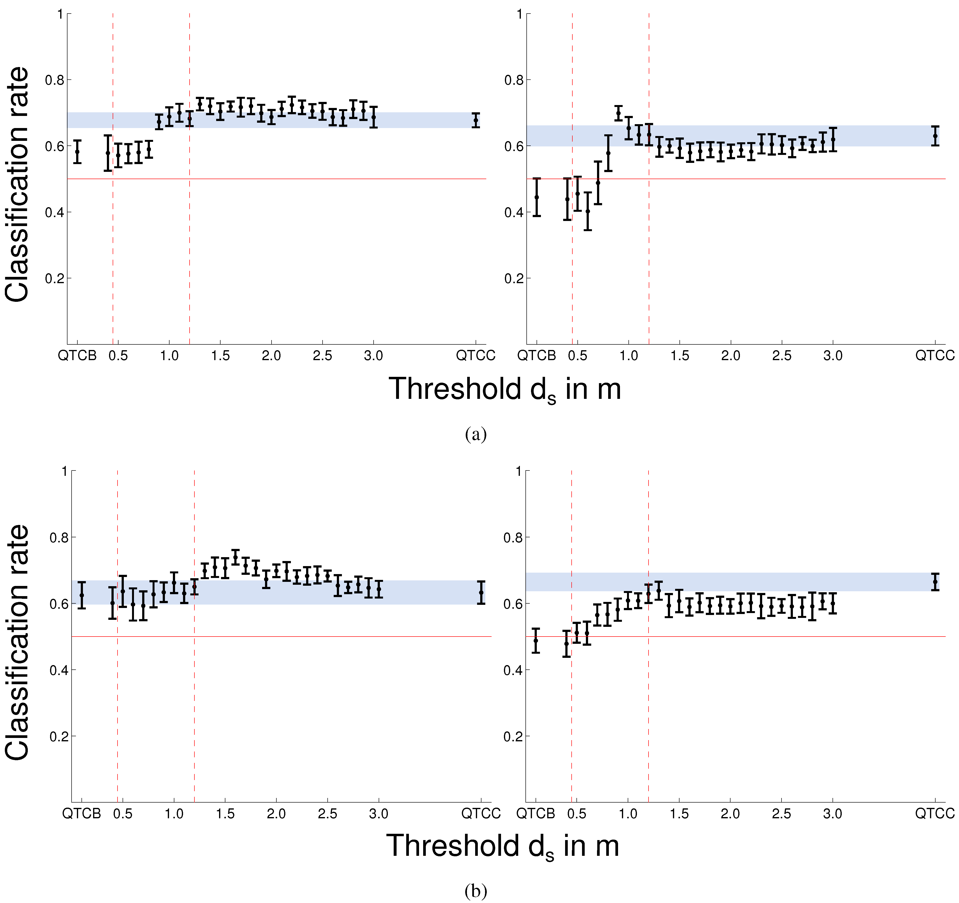
Left vs. Right The comparison of left
vs. right pass-by actions in both experiments shows that using pure
does, not surprisingly, yield bad results because the most important information–on which side the robot and the human pass by each other–is completely omitted in this 1-dimensional representation. Hence, all the classification results show that an increase in information about the 2-tuple
representing the 2D movement increases the performance of the classification. On the other hand, the results of both experiments show that the largest increase in performance of the classifier happens at distances of
0.7 m and that classification reaches
quality at
1.5 m (see yellow area in
Figure 12a,
Figure 13a and
Figure 15), which loosely resembles the area created by the far phase of Hall’s personal space and the close phase of the social space [
8]. These results could stem from the fact that the personal space was neither violate by the robot–be it fake or real–nor the participant. Judging from our data, the results indicate that information about the side
is most important if both agents enter, or are about to enter, each others personal spaces as can be seen from the yellow areas in
Figure 12a,
Figure 13a and
Figure 15. The information before crossing this threshold can be disregarded and is not important for the reliable classification of these two behaviours. As mentioned in our requirements, recognising the intention of the other interactant is a very important factor in the analysis of HRSI. Reducing the information about the side constraint and only regarding it when close together, allows to focus on the part of the interaction where both agents influence each others paths and therefore facilitates intention recognition, based on spatial movement.
Figure 15 shows that our model gives consistent results over the two experiments in the left
vs. right condition which is the only one we could compare in both. The blue curve shows the classification results for the “Lincoln experiment” whereas the green curve shows the results for the “Bristol experiment”. Both curves show the same trends of significantly increasing classification results from 0.7 m
1.5 m reaching their pinnacle at 1.5 m
2.0 m. This implies that our model is valid for this type of interaction regardless of the actual environment set-up and that the fact that we used an autonomous robot in one of the experiments and a “fake robot” in the other does not influence the data. More importantly, it also shows a suitable distance range for this kind of HRSI that also encloses all the other found distance ranges from the other conditions and is therefore a suitable candidate for
transitions.
Adaptive vs. Non-Adaptive Velocity Control Using a probabilistic model of pure
(as attempted in [
13]), it was not possible to reliably distinguish between the two behaviours the robot showed during the “Lincoln experiment”,
i.e., adaptive
vs. non-adaptive velocity control. We investigated if
would sufficiently highlight the part of the interaction that contains the most prominent difference between these two classes to enable a correct classification. Indeed, the results indicate that using a very low distance threshold
enables
to distinguish between these two cases for some of the smoothing levels. In
Figure 12b on the left side you can see the results from our previous work (using only pure
) [
13] visualised by a horizontal blue area. The Figure also shows that some of the
results are significantly different from
. Like for head-on
vs. overtake, the main difference between the adaptive and non-adaptive behaviour seems to lie in the
2-tuple,
i.e., both approach each other
vs. human approaches and robot stops
. On the other hand, the classification rate drops to
(
) at
1.3 m most likely due to the increase in noise. Nevertheless, apart from these typical results, there is also an interesting example where this does not hold true and we see a slight increase in classification rate at
1.5 m which was the stopping distance of the robot (see
Figure 12b, right). This shows that, even with
, the results for adaptive
vs. non-adaptive seem to be very dependent on the smoothing parameters (see
Table 1c) and therefore this problem still cannot be considered solved. Incorporating another HRSI concept,
i.e., velocity or acceleration, might be able to support modelling of these kind of behaviours.
Early vs. Late Looking at the data gathered in the “Bristol experiment”, we also evaluated early
vs. late (see
Figure 13b) avoidance manoeuvres. Just to recapitulate, early means the “robot” executed the avoidance manoeuvre 700 ms before the indicator and in the late condition 700 ms after. The data shows that our model is able to represent this kind of interaction for distances of 0.8 m
1.3 m. This is the distance the participants kept to the robot/experimenter in both experiments and loosely resembles Hall’s personal space [
8]. In this regard these results are consistent with the other described interactions showing that participants tried to protect their personal/intimate space. Except for the unsmoothed evaluation, we only achieved reliable classification using
inside the mentioned range of 0.8 m
1.3 m.
or
alone did not highlight the meaningful parts of the interaction and did not yield reliable results. Regarding the unsmoothed case, the fact that all the smoothing levels resulted in a significantly worse
classification than in the unsmoothed case shows that the unsmoothed result is most likely caused by artefacts due to minute movements before the start or after the end of the experiment. These movements cannot be regarded as important for the actual interaction and must therefore be considered unwanted noise.
Indicator vs. No Indicator The “Bristol experiment” also used indicators (be it flashing lights or cartoon eyes) to highlight the side the “robot” would move to. In the control condition no indicators were used. Modelling these two conditions we can see from the late condition that for 0.9 m, which resembles the mean minimum distance kept by the participant, we can reliably distinguish the two cases. The classification rate does not improve significantly for greater distances or pure but we are always able to reliably classify these two conditions. Compared to at 0.9 m, pure shows worse results for some of the smoothing levels. This indicates that the most important part of the interaction happens at close distances (the mean minimum distance of both agents 0.9 m) and adding more information does not increase the accuracy of the representation or even decreases it.
8. Conclusions
In this work we presented a HMM-based probabilistic sequential representation of HRSI utilising QTC, investigated the possibility of incorporating distances like the concept of proxemics [
8] into the model, and learned transitions in our combined QTC model and ranges of distances to trigger them, from real-world data. The data from our two experiments provides strong evidence regarding the generalisability and appropriateness of the representation, demonstrated by using it to classify different encounters observed in motion-capture data. We thereby created a tractable and concise representation that is general enough to abstract from metric space but rich enough to unambiguously model the observed spatial interactions between human and robot.
Using two different experiments, we have shown that, regardless of the modelled interaction type, our probabilistic sequential model using QTC is able to reliably classify most of the encounters. However, there are certain distances after which the “richer” 2D
encoding about the side constraint does not enhance the classification and thereby becomes irrelevant for the representation of the encounter. Hence,
’s 1D distance constraint is sufficient to model these interactions when the agents are far apart. On the other hand, we have seen that there are distances at which information about the side constraint becomes crucial for the description of the interaction like in passing on the left
vs. passing on the right. Thus, we found that there are intervals of distances between robot and human in which a switch to the 2-dimensional
model is necessary to represent HRSI encounters. These found distance intervals resemble the area of the far phase of Hall’s personal space and the close phase of the social space,
i.e., 0.76 m to 2.1 m [
8] (see
Figure 15). Therefore, our data shows that using the full 2D representation of
is unnecessary when the agents are further apart than the close phase of the social space (≈2.1 m) and can therefore be omitted. This not only creates a more compact representation but also highlights the interaction in close vicinity of the robot, modelling the essence of the interaction. Our results indicate that this
model is a valid representation of HRSI encounters and reliably describes the real-world interactions in the presented experiments.
As a welcome side effect of modelling distance using , our results show that the quality of the created probabilistic model is, in some cases, even increased compared to pure or . Thereby, besides allowing the representation of distance and the reduction of noise, it also enhances the representational capabilities of the model for certain distance values and outperforms pure . This shows the effect of reducing noise by filtering “unnecessary” information and focusing on the essence of the interaction.
Coming back to the four requirements to a model of HRSI stated in the introduction which were to
Represent the qualitative character of motions to recognise intention,
represent the main concepts of HRSI like proxemics [
8],
be able to generalise to facilitate knowledge transfer, and devise a
tractable, concise, and theoretically well-found model,
we have shown that our sequential model utilising
is able to achieve most of these. We exclusively implemented proxemics in our model which leaves room for improvement, incorporating other social norms, but shows that such a combination is indeed possible. Additionally, our representation is not only able to model
and
but also the proposed combination of both,
i.e.,
, which relies on the well founded original variants of the calculus. Therefore, the probabilistic sequential model based on
allows to implicitly represent one of the main concepts of HRSI, distances. We do so by combining the different variants of the calculus,
i.e., the mentioned
and
, into one integrated model. The resulting representation is able to highlight the interaction when the agents are in close vicinity to one another, allowing to focus on the qualitative character of the movement and therefore facilitates intention recognition. By eliminating information about the side the agents are moving to when far apart, we also create a more concise and tractable representation. Moreover, the model also inherits all the generalisability a qualitative representation offers. This is a first step to employ learned qualitative representations of HRSI for the generation and analysis of appropriate robot behaviour.
Concluding from the above statements, the probabilistic model of
is able to qualitatively model the observed interactions between two agents, abstracting from the metric 2D-space most other representations use, and implicitly incorporates the modelling of distance thresholds which, from the observations made in our experiments, represent one of the main social measures used in modern HRSI, proxemics [
8].
9. Future Work
This research was undertaken as part of an ongoing project (the STRANDS project [
48]) for which it will be used to generate appropriate HRSI behaviour based on previously observed encounters. The presented model will therefore be turned into a generative model to create behaviour as the basis for an online shaping framework for an autonomous robot. As part of this project, the robot is going to be deployed in an elder care home and an office building for up to 120 days continuously, able to collect data about the spatial movement of humans in real work environments.
To represent the interesting distance intervals we found in a more qualitative way, we will investigate possible qualitative spatial relations, e.g., close and far, ranging over the found interval of distances, instead of fixed thresholds. This will also be based on a probabilistic model using increasing transition probabilities depending on the current distance and the distance interval used. For example transitioning from to would be more likely the closer the actual distance is to the lower bound of the learned interval and vice-versa. In a generative system this will introduce variation and enables the learning of these distance thresholds.
To further improve this representation, we will work on a generalised version of our presented to deal with different and possibly multiple variants of QTC, which are not restricted to and , based also on other metrics beside Hall’s social distances to allow behaviour analysis and generation according to multiple HRSI measures.
The experiments we used were originally meant to investigate different aspects of HRSI and not to evaluate our model explicitly. Some of the more interesting phenomena in the experiments, especially the “Bristol Experiment”, like if the indicators had an effect on the interaction between the two agents or if the timing was important for the use of the indicators, will be investigated in more psychology focused work.


